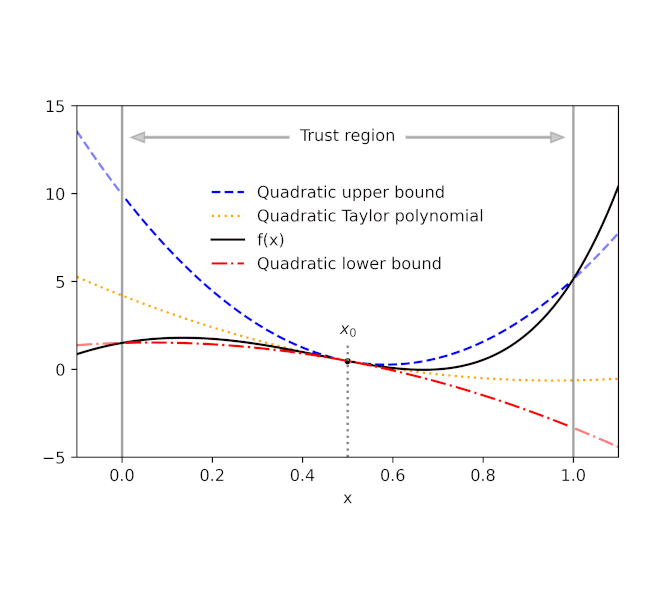
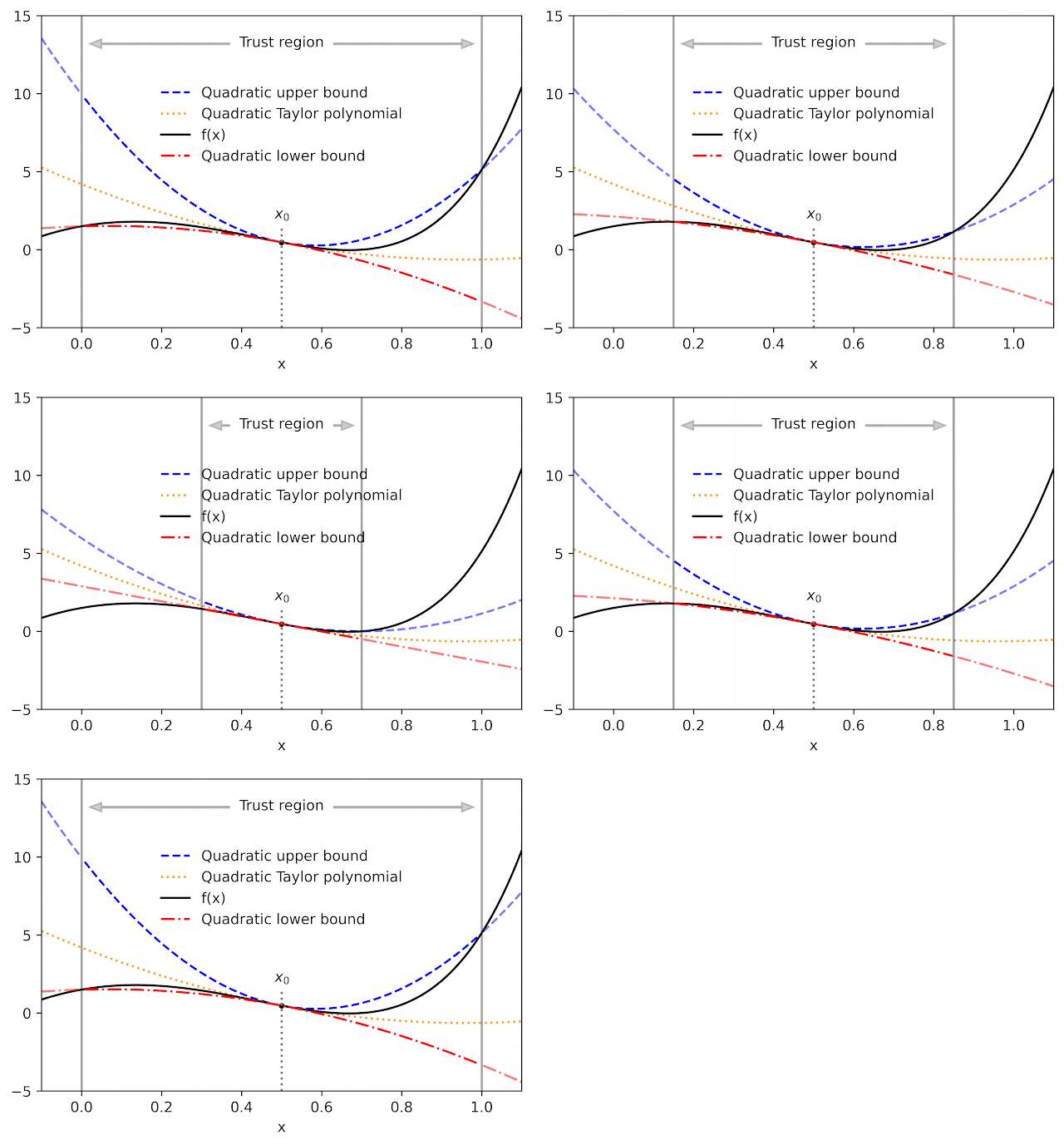
Beyond automatic differentiation

Posted by Matthew Streeter, Software Engineer, Google Research

Derivatives play a central role in optimization and machine learning. By locally approximating a training loss, derivatives guide an optimizer toward lower values of the loss. Automatic differentiation frameworks such as TensorFlow, PyTorch, and JAX are an essential part of modern machine learning, making it feasible to use gradient-based optimizers to train very complex models.

But are derivatives all we need? By themselves, derivatives only tell us how a function behaves on an infinitesimal scale. To use derivatives effectively, we often need to know more than that. For example, to choose a learning rate for gradient descent, we need to know something about how the loss function behaves over a small but finite window. A finite-scale analogue of automatic differentiation, if it existed, could help us make such choices more effectively and thereby speed up training.

In our new paper “Automatically Bounding The Taylor Remainder Series: Tighter Bounds and New Applications“, we present an algorithm called AutoBound that computes polynomial upper and lower bounds on a given function, which are valid over a user-specified interval. We then begin to explore AutoBound’s applications. Notably, we present a meta-optimizer called SafeRate that uses the upper bounds computed by AutoBound to derive learning rates that are guaranteed to monotonically reduce a given loss function, without the need for time-consuming hyperparameter tuning. We are also making AutoBound available as an open-source library.

The AutoBound algorithm

Given a function f and a reference point x₀, AutoBound computes polynomial upper and lower bounds on f that hold over a user-specified interval called a trust region. Like Taylor polynomials, the bounding polynomials are equal to f at x₀. The bounds become tighter as the trust region shrinks, and approach the corresponding Taylor polynomial as the trust region width approaches zero.

Automatically-derived quadratic upper and lower bounds on a one-dimensional function f, centered at x₀=0.5. The upper and lower bounds are valid over a user-specified trust region, and become tighter as the trust region shrinks.

Like automatic differentiation, AutoBound can be applied to any function that can be implemented using standard mathematical operations. In fact, AutoBound is a generalization of Taylor mode automatic differentiation, and is equivalent to it in the special case where the trust region has a width of zero.

To derive the AutoBound algorithm, there were two main challenges we had to address:

We had to derive polynomial upper and lower bounds for various elementary functions, given an arbitrary reference point and arbitrary trust region.
We had to come up with an analogue of the chain rule for combining these bounds.

Bounds for elementary functions

For a variety of commonly-used functions, we derive optimal polynomial upper and lower bounds in closed form. In this context, “optimal” means the bounds are as tight as possible, among all polynomials where only the maximum-degree coefficient differs from the Taylor series. Our theory applies to elementary functions, such as exp and log, and common neural network activation functions, such as ReLU and Swish. It builds upon and generalizes earlier work that applied only to quadratic bounds, and only for an unbounded trust region.

Optimal quadratic upper and lower bounds on the exponential function, centered at x₀=0.5 and valid over the interval [0, 2].

A new chain rule

To compute upper and lower bounds for arbitrary functions, we derived a generalization of the chain rule that operates on polynomial bounds. To illustrate the idea, suppose we have a function that can be written as

f(x) = g(h(x))

and suppose we already have polynomial upper and lower bounds on g and h. How do we compute bounds on f?

The key turns out to be representing the upper and lower bounds for a given function as a single polynomial whose highest-degree coefficient is an interval rather than a scalar. We can then plug the bound for h into the bound for g, and convert the result back to a polynomial of the same form using interval arithmetic. Under suitable assumptions about the trust region over which the bound on g holds, it can be shown that this procedure yields the desired bound on f.

The interval polynomial chain rule applied to the functions h(x) = sqrt(x) and g(y) = exp(y), with x₀=0.25 and trust region [0, 0.5].

Our chain rule applies to one-dimensional functions, but also to multivariate functions, such as matrix multiplications and convolutions.

Propagating bounds

Using our new chain rule, AutoBound propagates interval polynomial bounds through a computation graph from the inputs to the outputs, analogous to forward-mode automatic differentiation.

Forward propagation of interval polynomial bounds for the function f(x) = exp(sqrt(x)). We first compute (trivial) bounds on x, then use the chain rule to compute bounds on sqrt(x) and exp(sqrt(x)).

To compute bounds on a function f(x), AutoBound requires memory proportional to the dimension of x. For this reason, practical applications apply AutoBound to functions with a small number of inputs. However, as we will see, this does not prevent us from using AutoBound for neural network optimization.

Automatically deriving optimizers, and other applications

What can we do with AutoBound that we couldn’t do with automatic differentiation alone?

Among other things, AutoBound can be used to automatically derive problem-specific, hyperparameter-free optimizers that converge from any starting point. These optimizers iteratively reduce a loss by first using AutoBound to compute an upper bound on the loss that is tight at the current point, and then minimizing the upper bound to obtain the next point.

Minimizing a one-dimensional logistic regression loss using quadratic upper bounds derived automatically by AutoBound.

Optimizers that use upper bounds in this way are called majorization-minimization (MM) optimizers. Applied to one-dimensional logistic regression, AutoBound rederives an MM optimizer first published in 2009. Applied to more complex problems, AutoBound derives novel MM optimizers that would be difficult to derive by hand.

We can use a similar idea to take an existing optimizer such as Adam and convert it to a hyperparameter-free optimizer that is guaranteed to monotonically reduce the loss (in the full-batch setting). The resulting optimizer uses the same update direction as the original optimizer, but modifies the learning rate by minimizing a one-dimensional quadratic upper bound derived by AutoBound. We refer to the resulting meta-optimizer as SafeRate.

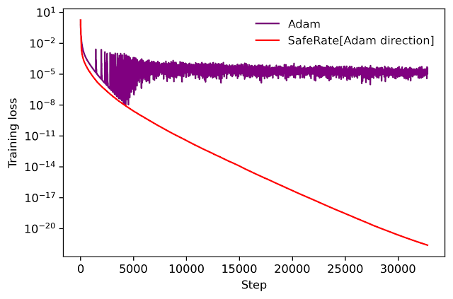Performance of SafeRate when used to train a single-hidden-layer neural network on a subset of the MNIST dataset, in the full-batch setting.

Using SafeRate, we can create more robust variants of existing optimizers, at the cost of a single additional forward pass that increases the wall time for each step by a small factor (about 2x in the example above).

In addition to the applications just discussed, AutoBound can be used for verified numerical integration and to automatically prove sharper versions of Jensen’s inequality, a fundamental mathematical inequality used frequently in statistics and other fields.

Improvement over classical bounds

Bounding the Taylor remainder term automatically is not a new idea. A classical technique produces degree k polynomial bounds on a function f that are valid over a trust region [a, b] by first computing an expression for the kth derivative of f (using automatic differentiation), then evaluating this expression over [a,b] using interval arithmetic.

While elegant, this approach has some inherent limitations that can lead to very loose bounds, as illustrated by the dotted blue lines in the figure below.

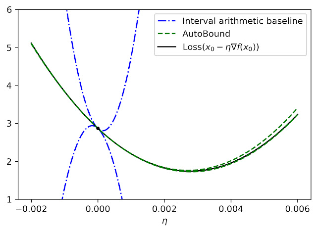Quadratic upper and lower bounds on the loss of a multi-layer perceptron with two hidden layers, as a function of the initial learning rate. The bounds derived by AutoBound are much tighter than those obtained using interval arithmetic evaluation of the second derivative.

Looking forward

Taylor polynomials have been in use for over three hundred years, and are omnipresent in numerical optimization and scientific computing. Nevertheless, Taylor polynomials have significant limitations, which can limit the capabilities of algorithms built on top of them. Our work is part of a growing literature that recognizes these limitations and seeks to develop a new foundation upon which more robust algorithms can be built.

Our experiments so far have only scratched the surface of what is possible using AutoBound, and we believe it has many applications we have not discovered. To encourage the research community to explore such possibilities, we have made AutoBound available as an open-source library built on top of JAX. To get started, visit our GitHub repo.